Subsetting, resampling, reprojection
Raster resampling/resizing
# run from the workshop data directory

$ gdal raster resize \
    SENTINEL2_L2A:S2B_MSIL2A_20260423T094029_N0512_R036_T34TER_20260423T115714.SAFE/MTD_MSIL2A.xml:10m:EPSG_32634 \
    10m_bands_to_20m.tif \
    --resolution 20,20 \
    --resampling cubic
or
$ gdal raster resize \
    SENTINEL2_L2A:S2B_MSIL2A_20260423T094029_N0512_R036_T34TER_20260423T115714.SAFE/MTD_MSIL2A.xml:10m:EPSG_32634 \
    10m_bands_half_size.tif \
    --size 50%,50% \
    --resampling cubic
Let's compare them with gdal raster compare
$ gdal raster compare 10m_bands_to_20m.tif 10m_bands_half_size.tif
==> no output, meaning they are bit-to-bit identical
Let's do that in Python
First,open a Python interpreter in the directory containing the workshop datasets:
$ python
Next, paste the following code snippet into the interpreter to perform the same operation as in the previous command-line example:
from osgeo import gdal
filename = "SENTINEL2_L2A:S2B_MSIL2A_20260423T094029_N0512_R036_T34TER_20260423T115714.SAFE/MTD_MSIL2A.xml:10m:EPSG_32634"
with gdal.alg.raster.resize(input=filename, output_format="MEM", output="", size=["50%","50%"]) as alg:
    output_dataset = alg.Output()
    print(output_dataset.ReadAsArray().shape)
(6, 5490, 5490)
Alternatively:
from osgeo import gdal
filename = "SENTINEL2_L2A:S2B_MSIL2A_20260423T094029_N0512_R036_T34TER_20260423T115714.SAFE/MTD_MSIL2A.xml:10m:EPSG_32634"
alg = gdal.Algorithm("raster", "resize")
alg["input"] = filename
alg["output_format"] = "MEM"
alg["output"] = ""
alg["size"]=["50%","50%"]
alg.Run()
output_dataset = alg.Output()
print(output_dataset.ReadAsArray().shape)
output_dataset.Close()  # needed when the output is a "real" file, to make sure it is closed
Clipping
Use gdal raster clip and gdal vector clip
$ gdal raster clip \
    SENTINEL2_L2A:S2B_MSIL2A_20260423T094029_N0512_R036_T34TER_20260423T115714.SAFE/MTD_MSIL2A.xml:10m:EPSG_32634 \
    clip.tif \
    --bbox 21.06809,45.64922,21.43590,45.86361 \
    --bbox-crs EPSG:4326
$ gdal vector clip timisoara.gpkg --layer points \
    timisoara_points_clipped.gpkg \
    --like clip.tif
Exercise
Clip SENTINEL2_L2A:S2B_MSIL2A_20260423T094029_N0512_R036_T34TER_20260423T115714.SAFE/MTD_MSIL2A.xml:10m:EPSG_32634
with a circle centered on Timișoara center (45.7558° N, 21.2322° E) with a radius of 1 km.
(hint)
Hint
Create a GeoJSON file with a single point with the center.
{"type":"Point", "coordinates":[<X>,<Y>]}
With
gdal vector info, note the name of the layerWith
gdal vector sql, create a circle centered around that geometry using options--sqland--dialect Spatialite, knowing that the geometry column name will begeometryand using SQL functionsST_Transformto reproject the coordinate to the EPSG code of the raster layer, andST_Bufferto create the circle.
Reprojection
Use gdal raster reproject and gdal vector reproject
$ gdal raster reproject s2_TDR_10m.xml --output-crs <TAB><TAB>
EPSG: ESRI: IAU_2015: IGNF: NKG: OGC: PROJ:
$ gdal raster reproject s2_TDR_10m.xml --output-crs EPSG:<TAB><TAB>
10659 -- ETRF2000 + EOMA 1980 height                     10596 -- WGS 84 / GLANCE Europe                          7902 -- ITRF90 (geographic 3D)
10660 -- HD72 / EOV + EOMA 1980 height                   27704 -- WGS 84 / Equi7 Europe                           7903 -- ITRF91 (geographic 3D)
23700 -- HD72 / EOV                                      4230 -- ED50 (geographic 2D)                             7904 -- ITRF92 (geographic 3D)
3819 -- HD1909 (geographic 2D)                           3034 -- ETRS89-extended / LCC Europe                     7905 -- ITRF93 (geographic 3D)
4237 -- HD72 (geographic 2D)                             3035 -- ETRS89-extended / LAEA Europe                    7906 -- ITRF94 (geographic 3D)
4075 -- SREF98 (geographic 2D)                           32234 -- WGS 72 / UTM zone 34N                           7907 -- ITRF96 (geographic 3D)
4074 -- SREF98 (geographic 3D)                           32434 -- WGS 72BE / UTM zone 34N                         7908 -- ITRF97 (geographic 3D)
8682 -- SRB_ETRS89 / UTM zone 34N                        32634 -- WGS 84 / UTM zone 34N                           8997 -- ITRF2000 (geographic 2D)
8685 -- SRB_ETRS89 (geographic 2D)                       3571 -- WGS 84 / North Pole LAEA Bering Sea              7909 -- ITRF2000 (geographic 3D)
8684 -- SRB_ETRS89 (geographic 3D)                       3572 -- WGS 84 / North Pole LAEA Alaska                  7910 -- ITRF2005 (geographic 3D)
6316 -- MGI 1901 / Balkans zone 7                        3573 -- WGS 84 / North Pole LAEA Canada                  7911 -- ITRF2008 (geographic 3D)
3836 -- Pulkovo 1942(83) / Gauss-Kruger zone 4           3574 -- WGS 84 / North Pole LAEA Atlantic                7912 -- ITRF2014 (geographic 3D)
31600 -- Dealul Piscului 1930 / Stereo 33                3575 -- WGS 84 / North Pole LAEA Europe                  8857 -- WGS 84 / Equal Earth Greenwich
4316 -- Dealul Piscului 1930 (geographic 2D)             3576 -- WGS 84 / North Pole LAEA Russia                  8888 -- WGS 84 (Transit) (geographic 2D)
3844 -- Pulkovo 1942(58) / Stereo70                      10598 -- WGS 84 / GLANCE North America                   8988 -- ITRF88 (geographic 2D)
3906 -- MGI 1901 (geographic 2D)                         27705 -- WGS 84 / Equi7 North America                    8989 -- ITRF89 (geographic 2D)
4805 -- MGI (Ferro) (geographic 2D)                      32600 -- WGS 84 / UTM grid system (northern hemisphere)  8990 -- ITRF90 (geographic 2D)
4178 -- Pulkovo 1942(83) (geographic 2D)                 3408 -- NSIDC EASE-Grid North                            8991 -- ITRF91 (geographic 2D)
3331 -- Pulkovo 1942(58) / 3-degree Gauss-Kruger zone 7  6931 -- WGS 84 / NSIDC EASE-Grid 2.0 North               8992 -- ITRF92 (geographic 2D)
3334 -- Pulkovo 1942(58) / Gauss-Kruger zone 4           3395 -- WGS 84 / World Mercator                          8993 -- ITRF93 (geographic 2D)
4179 -- Pulkovo 1942(58) (geographic 2D)                 3857 -- WGS 84 / Pseudo-Mercator                         8994 -- ITRF94 (geographic 2D)
7409 -- ETRS89 + EVRF2000 height                         3410 -- NSIDC EASE-Grid Global                           8995 -- ITRF96 (geographic 2D)
7423 -- ETRS89 + EVRF2007 height                         6933 -- WGS 84 / NSIDC EASE-Grid 2.0 Global              8996 -- ITRF97 (geographic 2D)
9422 -- ETRS89 + EVRF2019 height                         10178 -- IGS20 (geographic 2D)                           8998 -- ITRF2005 (geographic 2D)
9423 -- ETRS89 + EVRF2019 mean-tide height               10177 -- IGS20 (geographic 3D)                           8999 -- ITRF2008 (geographic 2D)
25834 -- ETRS89 / UTM zone 34N                           10345 -- Hughes 1980 (geographic 2D)                     9000 -- ITRF2014 (geographic 2D)
3046 -- ETRS89 / UTM zone 34N (N-E)                      10346 -- NSIDC Authalic Sphere (geographic 2D)           9003 -- IGS97 (geographic 2D)
23034 -- ED50 / UTM zone 34N                             10606 -- WGS 84 (G2296) (geographic 2D)                  9002 -- IGS97 (geographic 3D)
4231 -- ED87 (geographic 2D)                             10605 -- WGS 84 (G2296) (geographic 3D)                  9006 -- IGS00 (geographic 2D)
4668 -- ED79 (geographic 2D)                             10781 -- ITRF2020-u2023 (geographic 2D)                  9005 -- IGS00 (geographic 3D)
10571 -- ETRF2020 (geographic 2D)                        10780 -- ITRF2020-u2023 (geographic 3D)                  9009 -- IGb00 (geographic 2D)
10570 -- ETRF2020 (geographic 3D)                        10785 -- IGb20 (geographic 2D)                           9008 -- IGb00 (geographic 3D)
4258 -- ETRS89 (geographic 2D)                           10784 -- IGb20 (geographic 3D)                           9012 -- IGS05 (geographic 2D)
4937 -- ETRS89 (geographic 3D)                           4087 -- WGS 84 / World Equidistant Cylindrical           9011 -- IGS05 (geographic 3D)
9059 -- ETRF89 (geographic 2D)                           4276 -- NSWC 9Z-2 (geographic 2D)                        9014 -- IGS08 (geographic 2D)
7915 -- ETRF89 (geographic 3D)                           4322 -- WGS 72 (geographic 2D)                           9013 -- IGS08 (geographic 3D)
7917 -- ETRF90 (geographic 3D)                           4324 -- WGS 72BE (geographic 2D)                         9017 -- IGb08 (geographic 2D)
7919 -- ETRF91 (geographic 3D)                           4326 -- WGS 84 (geographic 2D)                           9016 -- IGb08 (geographic 3D)
7921 -- ETRF92 (geographic 3D)                           4740 -- PZ-90 (geographic 2D)                            9019 -- IGS14 (geographic 2D)
7923 -- ETRF93 (geographic 3D)                           4760 -- WGS 66 (geographic 2D)                           9018 -- IGS14 (geographic 3D)
7925 -- ETRF94 (geographic 3D)                           4891 -- WGS 66 (geographic 3D)                           9053 -- WGS 84 (G730) (geographic 2D)
7927 -- ETRF96 (geographic 3D)                           4923 -- PZ-90 (geographic 3D)                            9054 -- WGS 84 (G873) (geographic 2D)
7929 -- ETRF97 (geographic 3D)                           4979 -- WGS 84 (geographic 3D)                           9055 -- WGS 84 (G1150) (geographic 2D)
8399 -- ETRF2005 (geographic 3D)                         4985 -- WGS 72 (geographic 3D)                           9056 -- WGS 84 (G1674) (geographic 2D)
8403 -- ETRF2014 (geographic 3D)                         4987 -- WGS 72BE (geographic 3D)                         9057 -- WGS 84 (G1762) (geographic 2D)
9060 -- ETRF90 (geographic 2D)                           6893 -- WGS 84 / World Mercator + EGM2008 height         9380 -- IGb14 (geographic 2D)
9061 -- ETRF91 (geographic 2D)                           7657 -- WGS 84 (G730) (geographic 3D)                    9379 -- IGb14 (geographic 3D)
9062 -- ETRF92 (geographic 2D)                           7659 -- WGS 84 (G873) (geographic 3D)                    9474 -- PZ-90.02 (geographic 2D)
9063 -- ETRF93 (geographic 2D)                           7661 -- WGS 84 (G1150) (geographic 3D)                   9475 -- PZ-90.11 (geographic 2D)
9064 -- ETRF94 (geographic 2D)                           7663 -- WGS 84 (G1674) (geographic 3D)                   9518 -- WGS 84 + EGM2008 height
9065 -- ETRF96 (geographic 2D)                           7665 -- WGS 84 (G1762) (geographic 3D)                   9705 -- WGS 84 + MSL height
9066 -- ETRF97 (geographic 2D)                           7678 -- PZ-90.02 (geographic 3D)                         9707 -- WGS 84 + EGM96 height
9067 -- ETRF2000 (geographic 2D)                         7680 -- PZ-90.11 (geographic 3D)                         9755 -- WGS 84 (G2139) (geographic 2D)
7931 -- ETRF2000 (geographic 3D)                         7816 -- WGS 84 (Transit) (geographic 3D)                 9754 -- WGS 84 (G2139) (geographic 3D)
9068 -- ETRF2005 (geographic 2D)                         7900 -- ITRF88 (geographic 3D)                           9990 -- ITRF2020 (geographic 2D)
9069 -- ETRF2014 (geographic 2D)                         7901 -- ITRF89 (geographic 3D)                           9989 -- ITRF2020 (geographic 3D)
Or use CRS explorer at spatialreference.org
and let's write as a replayable .gdalg.json file:
https://gdal.org/en/stable/drivers/raster/gdalg.html
$ gdal raster scale TDR_rgb.tif TDR_rgb_byte_clamped.gdalg.json  \
        --input-min 400 \
        --input-max 2400 \
        --output-data-type uint8
$ cat TDR_rgb_byte_clamped.gdalg.json
{
  "type":"gdal_streamed_alg",
  "command_line":"gdal raster scale --input TDR_rgb.tif --output-data-type UInt8 --input-min 400 --input-max 2400 --output-format stream --output streamed_dataset",
  "gdal_version":"3130000"
}
$ gdal info TDR_rgb_byte_clamped.gdalg.json
Driver: GDALG/GDAL Streamed Algorithm driver
Files: TDR_rgb_byte_clamped.gdalg.json
Size is 10980, 10980
Coordinate Reference System:
  - name: WGS 84 / UTM zone 34N
  - ID: EPSG:32634
  - type: Projected
  - projection type: UTM zone 34N, Transverse Mercator
  - units: metre
  - area of use: Between 18°E and 24°E..., west 18.00, south 0.00, east 24.00, north 84.00
Data axis to CRS axis mapping: 1,2
Origin = (399960.000000000000000,5100000.000000000000000)
Pixel Size = (10.000000000000000,-10.000000000000000)
Metadata:
  AOT_QUANTIFICATION_VALUE=1000.0
  AOT_QUANTIFICATION_VALUE_UNIT=none
  AOT_RETRIEVAL_ACCURACY=0.0
  AOT_RETRIEVAL_METHOD=SEN2COR_DDV
  AREA_OR_POINT=Area
  BOA_QUANTIFICATION_VALUE=10000
  BOA_QUANTIFICATION_VALUE_UNIT=none
  CAST_SHADOW_PERCENTAGE=0.020978
  CLOUDY_PIXEL_OVER_LAND_PERCENTAGE=13.652931
  CLOUD_COVERAGE_ASSESSMENT=13.622445
  CLOUD_SHADOW_PERCENTAGE=4.0E-6
  DATATAKE_1_DATATAKE_SENSING_START=2026-04-23T09:40:29.024Z
  DATATAKE_1_DATATAKE_TYPE=INS-NOBS
  DATATAKE_1_ID=GS2B_20260423T094029_047681_N05.12
  DATATAKE_1_SENSING_ORBIT_DIRECTION=DESCENDING
  DATATAKE_1_SENSING_ORBIT_NUMBER=36
  DATATAKE_1_SPACECRAFT_NAME=Sentinel-2B
  DEGRADED_ANC_DATA_PERCENTAGE=0.0
  DEGRADED_MSI_DATA_PERCENTAGE=0
  FORMAT_CORRECTNESS=PASSED
  GENERAL_QUALITY=PASSED
  GENERATION_TIME=2026-04-23T11:57:14.000000Z
  GEOMETRIC_QUALITY=PASSED
  GRANULE_MEAN_AOT=0.06598
  GRANULE_MEAN_WV=0.75046
  HIGH_PROBA_CLOUDS_PERCENTAGE=0.001836
  L2A_QUALITY=PASSED
  MEDIUM_PROBA_CLOUDS_PERCENTAGE=0.009661
  NODATA_PIXEL_PERCENTAGE=9.990737
  NOT_VEGETATED_PERCENTAGE=28.988278
  OZONE_SOURCE=AUX_ECMWFT
  OZONE_VALUE=416.167104
  PREVIEW_GEO_INFO=Not applicable
  PREVIEW_IMAGE_URL=Not applicable
  PROCESSING_BASELINE=05.12
  PROCESSING_LEVEL=Level-2A
  PRODUCT_DOI=https://doi.org/10.5270/S2_-znk9xsj
  PRODUCT_START_TIME=2026-04-23T09:40:29.024Z
  PRODUCT_STOP_TIME=2026-04-23T09:40:29.024Z
  PRODUCT_TYPE=S2MSI2A
  PRODUCT_URI=S2B_MSIL2A_20260423T094029_N0512_R036_T34TDR_20260423T115714.SAFE
  RADIATIVE_TRANSFER_ACCURACY=0.0
  RADIOMETRIC_QUALITY=PASSED
  REFERENCE_BAND=B4
  REFLECTANCE_CONVERSION_U=0.991700831171221
  SATURATED_DEFECTIVE_PIXEL_PERCENTAGE=0.0
  SENSOR_QUALITY=PASSED
  SNOW_ICE_PERCENTAGE=0.0
  SPECIAL_VALUE_NODATA=0
  SPECIAL_VALUE_SATURATED=65535
  THIN_CIRRUS_PERCENTAGE=13.610949
  UNCLASSIFIED_PERCENTAGE=0.243549
  VEGETATION_PERCENTAGE=56.460464
  WATER_PERCENTAGE=0.664281
  WATER_VAPOUR_RETRIEVAL_ACCURACY=0.0
  WVP_QUANTIFICATION_VALUE=1000.0
  WVP_QUANTIFICATION_VALUE_UNIT=cm
Image Structure Metadata:
  INTERLEAVE=PIXEL
Corner Coordinates:
Upper Left  (  399960.000, 5100000.000) ( 19d42'25.02"E, 46d 2'46.53"N)
Lower Left  (  399960.000, 4990200.000) ( 19d43'45.90"E, 45d 3'29.49"N)
Upper Right (  509760.000, 5100000.000) ( 21d 7'34.20"E, 46d 3'12.62"N)
Lower Right (  509760.000, 4990200.000) ( 21d 7'26.31"E, 45d 3'54.69"N)
Center      (  454860.000, 5045100.000) ( 20d25'17.86"E, 45d33'28.71"N)
Band 1 Block=256x256 Type=Byte, ColorInterp=Red
  Metadata:
    BANDNAME=B4
    BANDWIDTH=30
    BANDWIDTH_UNIT=nm
    BOA_ADD_OFFSET=-1000
    SOLAR_IRRADIANCE=1512.79
    SOLAR_IRRADIANCE_UNIT=W/m2/um
    WAVELENGTH=665
    WAVELENGTH_UNIT=nm
Band 2 Block=256x256 Type=Byte, ColorInterp=Green
  Metadata:
    BANDNAME=B3
    BANDWIDTH=35
    BANDWIDTH_UNIT=nm
    BOA_ADD_OFFSET=-1000
    SOLAR_IRRADIANCE=1824.93
    SOLAR_IRRADIANCE_UNIT=W/m2/um
    WAVELENGTH=560
    WAVELENGTH_UNIT=nm
Band 3 Block=256x256 Type=Byte, ColorInterp=Blue
  Metadata:
    BANDNAME=B2
    BANDWIDTH=65
    BANDWIDTH_UNIT=nm
    BOA_ADD_OFFSET=-1000
    SOLAR_IRRADIANCE=1959.75
    SOLAR_IRRADIANCE_UNIT=W/m2/um
    WAVELENGTH=490
    WAVELENGTH_UNIT=nm
$ gdal raster reproject TDR_rgb_byte_clamped.gdalg.json TDR_3035.tif \
    --output-crs EPSG:3035 -r cubic --creation-option TILED=YES --creation-option COMPRESS=JPEG
Let's look at it in QGIS.
Nice, but can we get rid of the black collar ?
Sure let's say the nodata value (invalid value, sentinel value) to zero.
$ gdal raster edit TDR_3035.tif --nodata 0
Note
gdal raster edit is a bit of an exception in that it does not take an
input and output dataset, but a single one. The "edit" wording should make
it clear that this is edition in place.
Let's look again in QGIS. Zoom in on the south-western border. Hum "interesting" artifacts appear.
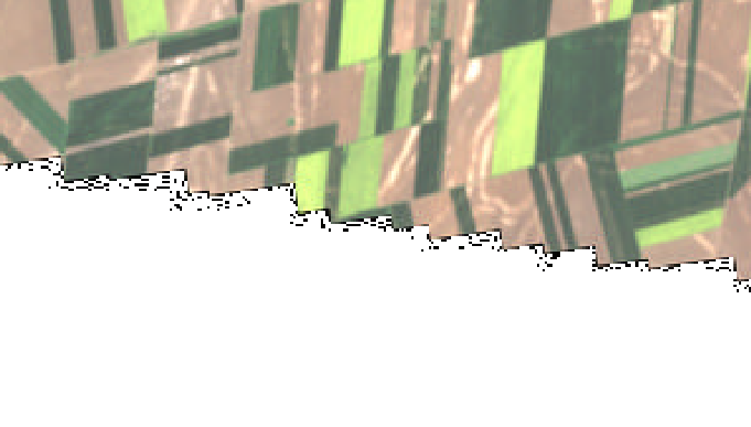
Let's clean them with gdal raster clean-collar
$ gdal raster clean-collar TDR_3035.tif TDR_3035_with_mask.tif \
    --add-mask --creation-option TILED=YES  --creation-option COMPRESS=JPEG
Exercise
Generate in a single step a tiled JPEG-compressed GeoTIFF reprojected image.
And make sure it includes overviews.
(hint)
Hint
Use the
--input-nodataand--add-alphaoptionsUse gdal raster overview add or use a format whose generation with GDAL automatically includes overviews.