DEM, VSI and nested pipelines
Failed attempt at getting a remote DEM
Let's find a DEM:
https://ec.europa.eu/eurostat/web/gisco/geodata/digital-elevation-model/eu-dem
$ gdal vsi ls -l /vsicurl/https://gisco-services.ec.europa.eu/dem/100k/EU_DEM_mosaic_1000K.ZIP
---------- 1 unknown unknown 25648052226 1970-01-01 00:00 /vsicurl/https://gisco-services.ec.europa.eu/dem/100k/EU_DEM_mosaic_1000K.ZIP
25 GB... hum
Note
If you are using the MSYS2 on Windows environment, you may see the error below:
ERROR 3: list: 'C:\gdal\msys64\vsicurl\https;\\gisco-services.ec.europa.eu\dem\100k\EU_DEM_mosaic_1000K.ZIP' does not exist or cannot be accessed
This is caused by MSYS2 path conversion (see https://www.msys2.org/docs/filesystem-paths/), which rewrites the URL passed to GDAL and breaks /vsicurl/. Fix it by disabling path conversion for the rest of this tutorial session with:
$ export MSYS_NO_PATHCONV=1
Let's have a look inside:
$ gdal vsi ls -l /vsizip/vsicurl/https://gisco-services.ec.europa.eu/dem/100k/EU_DEM_mosaic_1000K.ZIP
---------- 1 unknown unknown  24145219947 2013-10-02 19:55 eudem_dem_3035_europe.tif
---------- 1 unknown unknown   2374678674 2013-10-02 16:06 eudem_dem_3035_europe.tif.ovr
---------- 1 unknown unknown       290568 2013-10-16 10:16 metadata_iso19139.pdf
---------- 1 unknown unknown        18269 2013-10-16 10:00 metadata_iso19139.xml
---------- 1 unknown unknown         2836 2013-11-04 11:27 readme.txt
Let's be brave and inspect that huge TIFF file:
$ gdal info /vsizip/vsicurl/https://gisco-services.ec.europa.eu/dem/100k/EU_DEM_mosaic_1000K.ZIP/eudem_dem_3035_europe.tif
Driver: GTiff/GeoTIFF
[ ... takes forever ... ]
If that file had not been a compressed file (that is not using ZIP deflate compression), that would have been just fine, but nothing we can do about bad choices of data producers.
Successful attempt
Fortunately https://github.com/OpenTopography/OT_BulkAccess_COGs/blob/main/OT_BulkAccessCOGs.ipynb provides a useful hint, with a VRT example:
$ gdal raster info --no-fl /vsicurl/https://opentopography.s3.sdsc.edu/raster/SRTM_GL1/SRTM_GL1_srtm.vrt
Driver: VRT/Virtual Raster
Size is 1296001, 417601
Coordinate Reference System:
  - name: WGS 84
  - ID: EPSG:4326
  - type: Geographic 2D
Data axis to CRS axis mapping: 2,1
Origin = (-180.000138888888898,60.000138888888891)
Pixel Size = (0.000277777777778,-0.000277777777778)
Corner Coordinates:
Upper Left  (-180.0001389,  60.0001389) (180d 0' 0.50"W, 60d 0' 0.50"N)
Lower Left  (-180.0001389, -56.0001389) (180d 0' 0.50"W, 56d 0' 0.50"S)
Upper Right ( 180.0001389,  60.0001389) (180d 0' 0.50"E, 60d 0' 0.50"N)
Lower Right ( 180.0001389, -56.0001389) (180d 0' 0.50"E, 56d 0' 0.50"S)
Center      (   0.0000000,   2.0000000) (  0d 0' 0.00"E,  2d 0' 0.00"N)
Band 1 Block=128x128 Type=Int16, ColorInterp=Gray
  NoData Value=-32768
Now we can selectively download DEM covering our 3 Sentinel 2 tiles with:
# run from the workshop data directory

$ gdal raster clip \
    /vsicurl/https://opentopography.s3.sdsc.edu/raster/SRTM_GL1/SRTM_GL1_srtm.vrt \
    dem.tif \
    --like s2.vrt \
    --co COMPRESS=LZW --co TILED=YES --co PREDICTOR=2 --overwrite
Other successful attempt (using /vsis3/)
From https://hub.openeo.org/, Copernicus Data Space Ecosystem / Collections / COPERNICUS_30 / Items, one reaches https://stac.dataspace.copernicus.eu/v1/collections/cop-dem-glo-30-dged-cog/items which shows that one provider has a self-hosted (at least not under Amazon URL) S3 bucket at https://eodata.dataspace.copernicus.eu, which requires creating an account and getting credentials as indicated in https://documentation.dataspace.copernicus.eu/APIs/S3.html
Documentation of GDAL S3 related configuration options at: https://gdal.org/en/stable/user/virtual_file_systems.html#vsis3-aws-s3-files
Let's list the bucket content
$ gdal vsi ls -l /vsis3/eodata \
    --config AWS_S3_ENDPOINT=https://eodata.dataspace.copernicus.eu \
    --config AWS_ACCESS_KEY_ID=$EODATA_AWS_ACCESS_KEY_ID \
    --config AWS_SECRET_ACCESS_KEY=$EODATA_AWS_SECRET_ACCESS_KEY \
    --config AWS_VIRTUAL_HOSTING=NO
d--------- 1 unknown unknown            0 1970-01-01 00:00 C3S
d--------- 1 unknown unknown            0 1970-01-01 00:00 CAMS
d--------- 1 unknown unknown            0 1970-01-01 00:00 CEMS
d--------- 1 unknown unknown            0 1970-01-01 00:00 CLMS
d--------- 1 unknown unknown            0 1970-01-01 00:00 CLMS_archive
d--------- 1 unknown unknown            0 1970-01-01 00:00 Envisat
d--------- 1 unknown unknown            0 1970-01-01 00:00 Envisat-ASAR
d--------- 1 unknown unknown            0 1970-01-01 00:00 Global-Mosaics
d--------- 1 unknown unknown            0 1970-01-01 00:00 Jason-3
d--------- 1 unknown unknown            0 1970-01-01 00:00 Landsat-5
d--------- 1 unknown unknown            0 1970-01-01 00:00 Landsat-7
d--------- 1 unknown unknown            0 1970-01-01 00:00 Landsat-8-ESA
d--------- 1 unknown unknown            0 1970-01-01 00:00 SMOS
d--------- 1 unknown unknown            0 1970-01-01 00:00 SRTM
d--------- 1 unknown unknown            0 1970-01-01 00:00 Sentinel-1
d--------- 1 unknown unknown            0 1970-01-01 00:00 Sentinel-1-RTC
d--------- 1 unknown unknown            0 1970-01-01 00:00 Sentinel-2
d--------- 1 unknown unknown            0 1970-01-01 00:00 Sentinel-3
d--------- 1 unknown unknown            0 1970-01-01 00:00 Sentinel-5P
d--------- 1 unknown unknown            0 1970-01-01 00:00 Sentinel-6
d--------- 1 unknown unknown            0 1970-01-01 00:00 auxdata
Hint
You can streamline the access to such buckets by setting the credentials in
a $HOME/.gdal/gdalrc file (or $USERPROFILE/.gdal/gdalrc
on Windows and MYSYS2 e.g. C:\Users\my_user_name\.gdal\gdalrc)
[credentials]

[.eodata]
path=/vsis3/eodata
AWS_ACCESS_KEY_ID=<your-access-key-id-here>
AWS_SECRET_ACCESS_KEY=<your-secret-access-key-here>
AWS_S3_ENDPOINT=https://eodata.dataspace.copernicus.eu
AWS_VIRTUAL_HOSTING=NO
and them simply access a DEM 1 degree x 1 degree tile with:
$ gdal raster info \
    /vsis3/eodata/auxdata/CopDEM_COG/copernicus-dem-30m/Copernicus_DSM_COG_10_N45_00_E021_00_DEM/Copernicus_DSM_COG_10_N45_00_E021_00_DEM.tif
Driver: GTiff/GeoTIFF
Files: /vsis3/eodata/auxdata/CopDEM_COG/copernicus-dem-30m/Copernicus_DSM_COG_10_N45_00_E021_00_DEM/Copernicus_DSM_COG_10_N45_00_E021_00_DEM.tif
Size is 3600, 3600
Coordinate Reference System:
  - name: WGS 84
  - ID: EPSG:4326
  - type: Geographic 2D
  - area of use: World, west -180.00, south -90.00, east 180.00, north 90.00
Data axis to CRS axis mapping: 2,1
Origin = (20.999861111111112,46.000138888888891)
Pixel Size = (0.000277777777778,-0.000277777777778)
Metadata:
  AREA_OR_POINT=Point
Image Structure Metadata:
  LAYOUT=COG
  COMPRESSION=DEFLATE
  INTERLEAVE=BAND
  PREDICTOR=3
Corner Coordinates:
Upper Left  (  20.9998611,  46.0001389) ( 20d59'59.50"E, 46d 0' 0.50"N)
Lower Left  (  20.9998611,  45.0001389) ( 20d59'59.50"E, 45d 0' 0.50"N)
Upper Right (  21.9998611,  46.0001389) ( 21d59'59.50"E, 46d 0' 0.50"N)
Lower Right (  21.9998611,  45.0001389) ( 21d59'59.50"E, 45d 0' 0.50"N)
Center      (  21.4998611,  45.5001389) ( 21d29'59.50"E, 45d30' 0.50"N)
Band 1 Block=1024x1024 Type=Float32, ColorInterp=Gray
  Overviews: 1800x1800, 900x900, 450x450
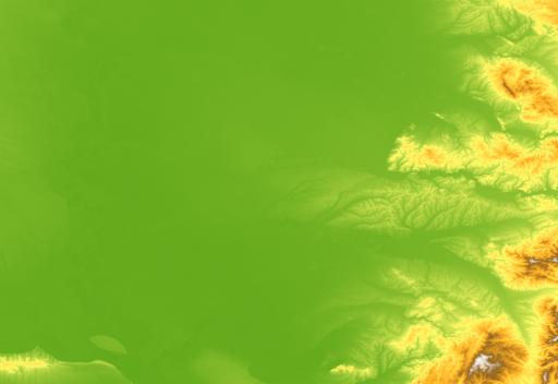
Hypsometric rendering
With gdal raster color-map.
and following color ramp placed in test.cpt (Source: "elevation1" from https://hub.qgis.org/styles/28/ ported from XML)
0%     74,156,15,255
25%    255,250,104,255
50%    255,179,38,255
75%    146,100,30,255
100%   255,255,255,255
nv     0,0,0,0
Note
Above is optimized for high contrast for the analyzed area. Not appropriate for comparing different regions with different elevation ranges.
$ gdal raster color-map dem.tif --color-map test.cpt dem_colorized.tif
Result:
Shaded map
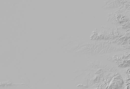
With gdal raster hillshade.
$ gdal raster hillshade dem.tif dem_hillshade.tif
Result:
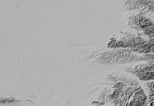
You can exaggerate the effect of altitudes to accentuate slopes
$ gdal raster hillshade dem.tif dem_hillshade_z_5.tif --zfactor 5
Result:
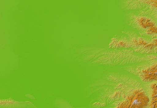
Combining hypsometric rendering and hillshade
With gdal raster blend.
$ gdal raster blend --color-input dem_colorized.tif \
        --overlay dem_hillshade.tif \
        --output dem_colorized_hillshade.tif \
        --operator hsv-value
Result:
You can adjust the opacity of the overlay layer:
$ gdal raster blend --color-input dem_colorized.tif \
        --overlay dem_hillshade.tif \
        --output dem_colorized_hillshade_50pct.tif \
        --operator hsv-value --opacity 50
Result:
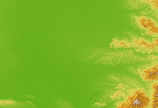
Doing it in one step: nested pipeline !
Using gdal raster pipeline,
and write is a .gdalg.json file
$ gdal raster pipeline \
    read dem.tif ! \
    color-map --color-map test.cpt ! \
    blend [ read dem.tif ! hillshade ] --operator hsv-value ! \
    write dem_pipeline.gdalg.json

And let's open it in QGIS.
Exercise
Modify the above pipeline:
such that the hillshade stage appears first and the
color-mapone is done as a nested input pipeline.
(hint)
Hint
Specify the hypsometric rendering with a nested input pipeline as the value
of the --input argument of blend and use the special
placeholder _PIPE_
to generate colorized and hillshaded maps as intermediate results
(hint)
Hint
Use the tee pipeline operator
You may also use it inside a nested input pipeline